Quickstart

Here we illustrate the basic usage of the adrt package as well as describe some of the transforms it implements. In the examples below, we will make use of a few basic Python libraries:

import numpy as np
from matplotlib import pyplot as plt
import adrt

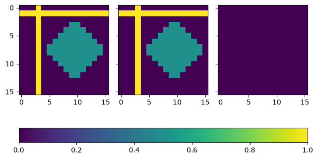
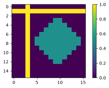
As a running example, we will operate on the image below.

# Generate image
n = 16
xs = np.linspace(-1, 1, n)
x, y = np.meshgrid(xs, xs)
img = 0.5 * ((np.abs(x - 0.25) + np.abs(y)) < 0.7).astype(np.float32)
img[:, 3] = 1
img[1, :] = 1

# Display
plt.figure(figsize=(5, 3))
plt.imshow(img)
plt.colorbar()
plt.tight_layout();

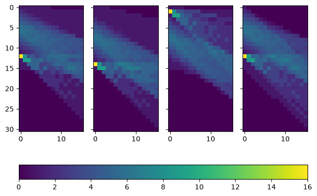
Forward Transform

The core transformation implemented in this package is the approximate discrete Radon transform (ADRT). The ADRT computes sums along discrete, digital lines at many angles which approximate sums along continuous lines in the image. At each angle, several lines are used, each crossing the edge of the input image at a different offset.

The angles are divided into quadrants each of which has a width of \(\pi/4\) radians. The angles for each quadrant are taken from a canonical range from \(-\pi/2\) through \(\pi/2\) starting from the negative side. In each quadrant the leftmost column contains lines which are either horizontal or vertical, and angles vary toward the diagonal angle for that quadrant in the rightmost column.

The offsets for each ADRT line change from row to row in each quadrant. The top row is always completely filled in, while the lower triangle is filled with zeros.

The figure in this section illustrates this structure. The function adrt.utils.coord_adrt() gives the angle and offset for each output entry.

An illustration of the lines along which ADRT sums are computed. The lines are drawn in red and their positions in the input image are shown against the light blue squares. Angles change across the columns of each quadrant, while offsets change across the rows.

The result of the ADRT can be computed for our sample image with adrt.adrt(). Compare the higher-valued entries against the structure of the sample image and the positions illustrated in the figure.

adrt_result = adrt.adrt(img)

# Display result
fig, axs = plt.subplots(1, 4, sharey=True)
for i, ax in enumerate(axs.ravel()):
    im_plot = ax.imshow(adrt_result[i], vmin=0, vmax=np.max(adrt_result))
fig.tight_layout()
fig.colorbar(im_plot, ax=axs, orientation="horizontal");

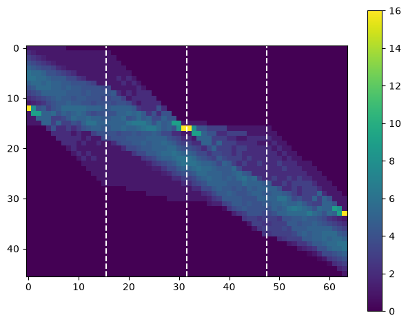
For illustration purposes this result can be stitched together using adrt.utils.stitch_adrt(). If desired, the result of the stitching operation can be undone with adrt.utils.unstitch_adrt().

adrt_stitched = adrt.utils.stitch_adrt(adrt_result)

# Display result
plt.imshow(adrt_stitched)
plt.colorbar()
for i in range(1, 4):
    plt.axvline(n * i - 0.5, color="white", linestyle="--")
plt.tight_layout();

Inverse Transforms

In the special case where the image has quantized values, the exact ADRT formula applies. This can be computed by adrt.iadrt(). Consult the reference for more information on available inverses and consider the recipe in the Iterative Inverse example for an inverse which may be more suitable for general use.

iadrt_out = adrt.iadrt(adrt_result)
iadrt_truncated = adrt.utils.truncate(iadrt_out)
iadrt_result = np.mean(iadrt_truncated, axis=0)

diff = iadrt_result - img

results = [img, iadrt_result, diff]

# Display
fig, axs = plt.subplots(1, 3, sharey=True)
for i, ax in enumerate(axs.ravel()):
    im_plot = ax.imshow(results[i], vmin=0, vmax=np.max(img))
fig.tight_layout()
fig.colorbar(im_plot, ax=axs, orientation="horizontal");