Sinograms of an Image
The discretized Radon transforms are often used to approximate sinograms of a
known image. adrt provides utilities that map the ADRT output which is
in the ADRT coordinates \((s, h)\) to a sinogram which is in the Cartesian
coordinates \((\theta, t)\).
We make use of this package as well as a few other fundamental libraries.
import numpy as np
from matplotlib import pyplot as plt
import adrt
We will illustrate the computation of sinograms with a few examples. The simple geometry relating the two coordinates \((s, h)\) and \((\theta, t)\) is detailed in the Coordinate Transform Section.
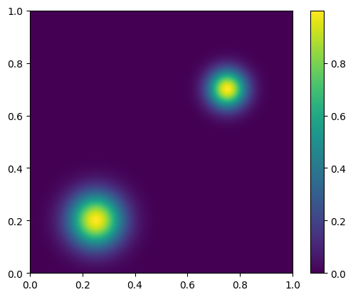
Gaussian Humps
We compute an image that is a sum of two Gaussian humps.
n = 2**9
x1 = np.linspace(0.0, 1.0, n)
X, Y = np.meshgrid(x1, x1)
s1 = 200
s2 = 100

gaussians = np.exp(-s1 * (X - 0.75) ** 2 - s1 * (Y - 0.3) ** 2) + np.exp(
    -s2 * (X - 0.25) ** 2 - s2 * (Y - 0.8) ** 2
)
plt.imshow(gaussians, extent=(0, 1, 0, 1))
plt.colorbar();
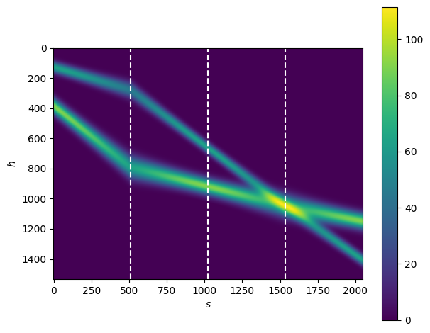
We compute the ADRT of this image and plot the image.
adrt_result = adrt.adrt(gaussians)
adrt_stitched = adrt.utils.stitch_adrt(adrt_result)

plt.imshow(adrt_stitched)
plt.colorbar()
for i in range(1, 4):
    plt.axvline(n * i - 0.5, color="white", linestyle="--")
plt.ylabel("$h$")
plt.xlabel("$s$")
plt.tight_layout();
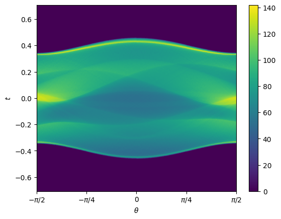
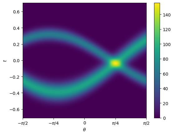
From the ADRT data we compute the sinogram by using the function
adrt.utils.interp_to_cart(). Each isotropic Gaussian hump corresponds to
a sinusoidal curve of commensurate width in the sinogram.
img_cart = adrt.utils.interp_to_cart(adrt_result)
img_extent = 0.5 * np.array([-np.pi, np.pi, -np.sqrt(2), np.sqrt(2)])

plt.imshow(img_cart, aspect="auto", extent=img_extent)
plt.colorbar()
plt.xticks(
    [-np.pi / 2, -np.pi / 4, 0, np.pi / 4, np.pi / 2],
    [r"$-\pi/2$", r"$-\pi/4$", "0", r"$\pi/4$", r"$\pi/2$"],
)
plt.ylabel("$t$")
plt.xlabel(r"$\theta$");
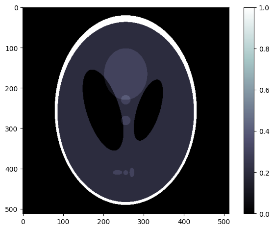
Shepp-Logan Phantom
As a more involved example we can consider the Shepp-Logan phantom
(data file).
phantom = np.load("data/shepp-logan.npz")["phantom"]
n = phantom.shape[0]

# Display the image
plt.imshow(phantom, cmap="bone")
plt.colorbar()
plt.tight_layout();
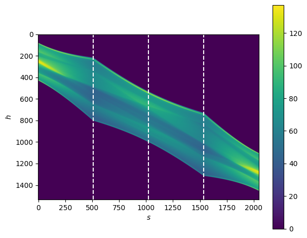
We can start by computing the ADRT of this image
adrt_result = adrt.adrt(phantom)
adrt_stitched = adrt.utils.stitch_adrt(adrt_result)

plt.imshow(adrt_stitched)
plt.colorbar()
for i in range(1, 4):
    plt.axvline(n * i - 0.5, color="white", linestyle="--")
plt.ylabel("$h$")
plt.xlabel("$s$")
plt.tight_layout();
These can be interpolated to a Cartesian grid with
adrt.utils.interp_to_cart().
img_cart = adrt.utils.interp_to_cart(adrt_result)
img_extent = 0.5 * np.array([-np.pi, np.pi, -np.sqrt(2), np.sqrt(2)])

plt.imshow(img_cart, aspect="auto", extent=img_extent)
plt.colorbar()
plt.xticks(
    [-np.pi / 2, -np.pi / 4, 0, np.pi / 4, np.pi / 2],
    [r"$-\pi/2$", r"$-\pi/4$", "0", r"$\pi/4$", r"$\pi/2$"],
)
plt.ylabel("$t$")
plt.xlabel(r"$\theta$");