Computerized Tomography
We can solve the Computerized Tomography (CT) problem using the
routines in adrt. For a detailed mathematical description,
see standard references[1] on the topic.
Here we will be using SciPy’s scipy.sparse.linalg.cg() routine as
illustrated in the Iterative Inverse Section. We first
import requisite modules then define the ADRTNormalOperator and the
function iadrt_cg. However, we modify the operator by adding to it a
multiple of the identity and name the new operator ADRTRidgeOperator below.
# Using ADRTNormalOperator from the Iterative Inverse example
class ADRTRidgeOperator(ADRTNormalOperator):
   def __init__(self, img_size, dtype=None, ridge_param=1000.0):
      super().__init__(dtype=dtype, img_size=img_size)
      self._ridge_param = ridge_param

   def _matmat(self, x):
      # Use batch dimensions to handle columns of matrix x
      return super()._matmat(x) + self._ridge_param * x
Using this operator with the CG algorithm yields the solution to the ridge
regression problem given by \((A^{T}A + \lambda I)x = A^{T}b\) where
\(A\) is the matrix representation of adrt.adrt(), \(I\) is the
identity matrix, and \(\lambda \ge 0\) is the ridge parameter.
Forward Data
For this demonstration, we will make use of synthetic forward
measurement data for the CT problem. We will attempt to recover the
Shepp-Logan phantom (data file)
from its Radon transform.
phantom = np.load("data/shepp-logan.npz")["phantom"]
n = phantom.shape[0]
We sample the CT data on a uniform Cartesian grid in the \((\theta, t)\)
coordinates using the routine provided in skimage.transform.radon().
from skimage.transform import radon

th_array1 = np.unique(adrt.utils.coord_adrt(n).angle)
theta = 90.0 + np.rad2deg(th_array1.squeeze())
sinogram = radon(phantom, theta=theta)
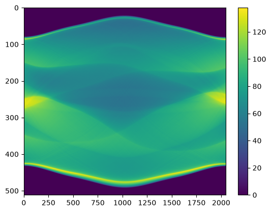
The sampled sinogram is plotted below. Although this sinogram appears similar to that in the sinogram computation example, there are differences: The grid in the \((\theta, t)\) coordinates used here is different, and the approximation used in discretizing the continuous transform is also different.
plt.imshow(sinogram, aspect="auto")
plt.colorbar();
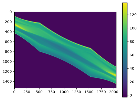
Then we use scipy.interpolate.RectBivariateSpline to
interpolate the sampled forward data at the ADRT coordinates, forming
the ADRT data. We plot the interpolated data below.
from scipy import interpolate

t_array = np.linspace(-0.5, 0.5, n)
spline = interpolate.RectBivariateSpline(t_array, th_array1, sinogram)
s_array, th_array = adrt.utils.coord_adrt(n)
adrt_data = spline(s_array, th_array, grid=False)

adrt_stitched = adrt.utils.stitch_adrt(adrt_data)
plt.imshow(adrt_stitched)
plt.colorbar();
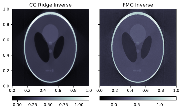
Inversion result
We turn to the solution of the ridge regression problem using the CG algorithm.
We also show the inverse computed with adrt.iadrt_fmg() included in the
package without any regularization for illustration and comparison.
# Using iadrt_cg from the Iterative Inverse example
cg_inv = iadrt_cg(adrt_data, op_cls=ADRTRidgeOperator)
fmg_inv = adrt.iadrt_fmg(adrt_data)

# Display inversion result
fig, axs = plt.subplots(1, 2, sharey=True)
for ax, data, title in zip(
    axs.ravel(),
    [cg_inv, fmg_inv],
    ["CG Ridge Inverse", "FMG Inverse"],
):
    im_plot = ax.imshow(data, cmap="bone", extent=(0, 1, 0, 1))
    fig.colorbar(im_plot, ax=ax, orientation="horizontal", pad=0.08)
    ax.set_title(title)
fig.tight_layout();
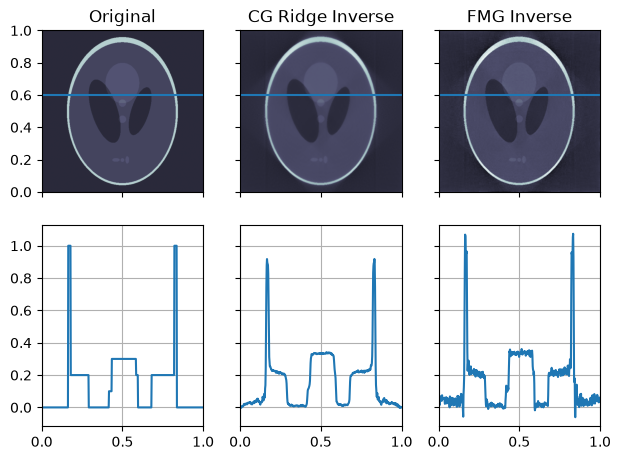
The inversion result, together with a slice plot in the horizontal direction, is displayed below.
fig, axs = plt.subplots(
    2, 3, sharex=True, sharey="row",
)
vmin = min(map(np.min, [phantom, cg_inv, fmg_inv]))
vmax = max(map(np.max, [phantom, cg_inv, fmg_inv]))
plot_row = n // 5 * 2
plot_x = np.linspace(0.0, 1.0, n)

for ax, data, title in zip(
    axs.T,
    [phantom, cg_inv, fmg_inv],
    ["Original", "CG Ridge Inverse", "FMG Inverse"],
):
    im_ax, plot_ax = ax
    im_ax.imshow(
        data,
        cmap="bone",
        extent=(0, 1, 0, 1),
        vmin=vmin,
        vmax=vmax,
    )
    im_ax.axhline(0.6, color="C0")
    im_ax.set_title(title)
    plot_ax.plot(plot_x, data[plot_row, :], "C0")
    plot_ax.grid(True)
fig.tight_layout();