Wave Equation
The Radon transform allows one to solve the multi-dimensional wave equation \(\partial_t^2 u = \Delta u\) by transforming the problem into a family of 1D wave equations in the Radon domain, due to its intertwining property.[1] As a result, one can solve the 1D wave equations in the Radon domain then transform back into the physical variables to obtain the solution. Note that this solution is essentially identical to the Lax-Philips translation representation.[2]
For this solution, we will need to invert the Radon transform: we will again be
using SciPy’s scipy.sparse.linalg.cg() routine as illustrated in the
Iterative Inverse Section and make use of the function
iadrt_cg from that example.
We choose a superposition of two cosine peaks as the initial condition and form its discretization.
n = 2**9
xx = np.linspace(0.0, 1.0, n)
X, Y = np.meshgrid(xx, xx)

alph1 = 16.0
alph2 = 8.0

x1, y1 = 0.6, 0.65
x2, y2 = 0.4, 0.35

R1 = np.sqrt((X - x1)**2 + (Y - y1)**2)
R2 = np.sqrt((X - x2)**2 + (Y - y2)**2)

init = 0.5*(np.cos(np.pi*alph1*R1) + 1.0)*(R1 < 1.0/alph1) \
     + 0.5*(np.cos(np.pi*alph2*R2) + 1.0)*(R2 < 1.0/alph2)
We then approximate the Radon transform of the initial condition using adrt.adrt().
init_adrt = adrt.adrt(init)
For each angular slice, we translate the initial condition following the d’Alembert formula.
sol_adrt = np.zeros(init_adrt.shape)

m = init_adrt.shape[1]

# Eulerian grid
yy = np.linspace(-1.0, 1.0, m)

time = 0.20
for q in range(4):
    for i in range(n):
        th = np.arctan(i/(n-1))

        # Construct Lagrangian grid then interpolate
        xx = yy + time/np.cos(th)
        sol_adrt[q, :, i] += 0.5*np.interp(yy, xx, init_adrt[q, :, i])
        xx = yy - time/np.cos(th)
        sol_adrt[q, :, i] += 0.5*np.interp(yy, xx, init_adrt[q, :, i])
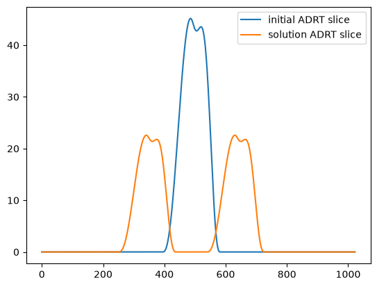
Finally, we plot the solution.
plt.plot(init_adrt[0, :, m//2], label="initial ADRT slice")
plt.plot(sol_adrt[0, :, m//2], label="solution ADRT slice")
plt.legend();
Finally, we invert the ADRT.
# Using iadrt_cg from the Iterative Inverse example
sol = iadrt_cg(sol_adrt)
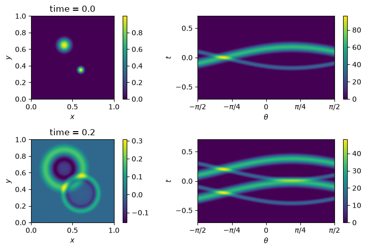
We plot the solution, and also show the Cartesian view of the ADRT data.
fig, axs = plt.subplots(nrows=2, ncols=2, figsize=(8, 5))

cart_extent = 0.5 * np.array([-np.pi, np.pi, -np.sqrt(2), np.sqrt(2)])

ax = axs[0, 1]
im = ax.imshow(adrt.utils.interp_to_cart(init_adrt), aspect="auto", extent=cart_extent)
plt.colorbar(im, ax=ax)
ax.set_xticks([ -np.pi/2,    -np.pi/4,   0,   np.pi/4,   np.pi/2],
              [r"$-\pi/2$", r"$-\pi/4$", "0", r"$\pi/4$", r"$\pi/2$"])
ax.set_xlabel(r"$\theta$")
ax.set_ylabel("$t$")

ax = axs[1, 1]
im = ax.imshow(adrt.utils.interp_to_cart(sol_adrt), aspect="auto", extent=cart_extent)
plt.colorbar(im, ax=ax)
ax.set_xticks([ -np.pi/2,    -np.pi/4,   0,   np.pi/4,   np.pi/2],
              [r"$-\pi/2$", r"$-\pi/4$", "0", r"$\pi/4$", r"$\pi/2$"])
ax.set_xlabel(r"$\theta$")
ax.set_ylabel("$t$")

ax = axs[0, 0]
im = ax.imshow(init, extent=(0, 1, 0, 1))
ax.set_title("time = 0.0")
plt.colorbar(im, ax=ax)
ax.set_aspect(1)
ax.set_xlabel("$x$")
ax.set_ylabel("$y$")

ax = axs[1, 0]
ax.set_title(f"time = {time:1.1f}")
im = ax.imshow(sol, extent=(0, 1, 0, 1))
plt.colorbar(im, ax=ax)
ax.set_aspect(1)
ax.set_xlabel("$x$")
ax.set_ylabel("$y$")

fig.tight_layout();